

Content Warning: Math, Handwaving
I spent a lot of time doodling in middle school in lieu of whatever it is middle schoolers are
supposed to be doing. Somewhere between the Cool S’s
and Penrose triangles I stumbled upon a neat
way to fill up graph paper by repeatedly combining and copying squares. I suspected there was
more to the doodle but wasn’t quite sure how to analyze it. Deciding to delegate to a future version of me that
knows more math, I put it up on the wall behind my desk where it has followed me from high
school to college to the present day.
Anyway, after a series of accidents I am now the prophesized future version of me that knows a bit more math.
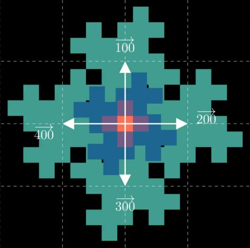
Due to its petal-like blooming structure and timeless presence scotch taped to my wall I’ll be referring to the
fractal affectionately as “the wallflower,” although further down we’ll see it’s closely related
to some well-known fractals. To start investigating it might help to run through
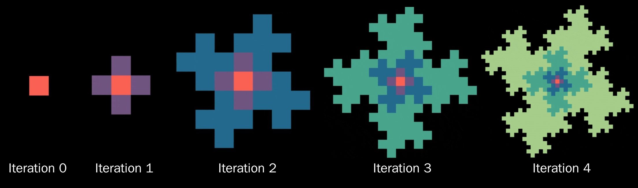
the steps of how middle school me originally drew it:
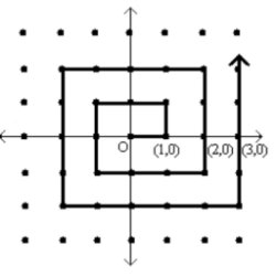
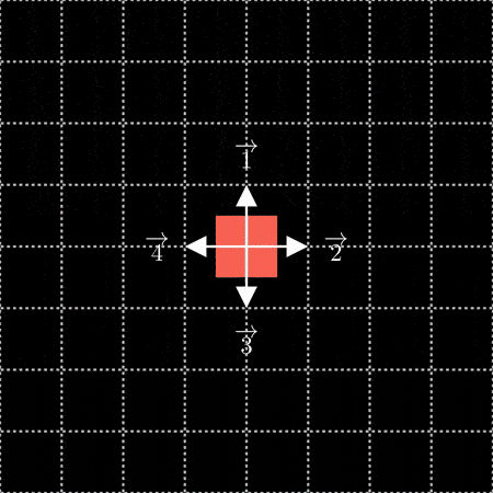
- Start with a single square.
- Tile four copies of the current state to the left, right, top, and bottom of the current state.
- Tile four copies of the current state slightly angled (about 27 degrees clockwise) from the left, right, top, and bottom of the current state.
- Alternate between steps 2 and 3 until you run out of graph paper.
In animated form:
Shoutout to manim and 3Blue1Brown for making this and many other visualizations to come possible!
Similar to the Gosper Curve, the steps can
be run repeatedly to eventually cover any part of the plane, and each intermediate state can tile the plane.
If you have graph paper and free time you can try out the steps for yourself – it’s fun to
translate and trace the contour of the previous state and watch things lock into place like a puzzle.
Alternatively, a bit over a year ago I realized you could
generate the contour using an L-System.
The rules are simple and consist of only 90 degree right ((R)) and left ((L)) turns:
- Start with 4 right turns: (RRRR)
- Each iteration run the following substitutions: (R rightarrow RLR, L rightarrow RLL)
For example, after applying the first iteration of substitutions you should have (RLRRLRRLRLR).
The following images demonstrate the first few applications of the rule:
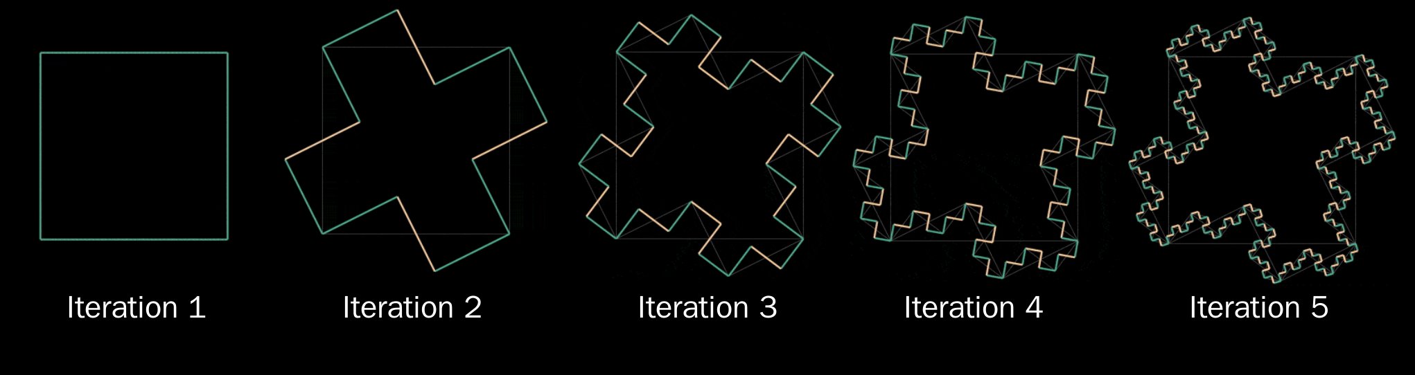
Yellow=next turn (going clockwise) will be to the left, Blue=to the right
And in animated form:

Both methods end up generating equivale– hold up! When I first tried
the L-System method a year ago I thought it generated the same contour as the wallflower.
In other words, I tried drawing the fourth iteration and its many right angles free
hand and gave up partway thinking “well it worked for the first 3 iterations, therefore it works in general (text{Q.E.D.})”
It was only when I started making the animations for this post that I realized
the two don’t quite match up. Comparing the 4th iteration from each method:

Side by side, the main difference between the two is how the “copies”
of the 3rd iteration are placed around the original in the center. The first method (let’s call it
“drag and drop”) places the copies directly above, below, etc… around the center, while
the L-System method places them diagonally. The contour produced by the L-System
approach is already documented in a few places:
- Wikipedia article for List of fractals (listed as “Quadratic von Koch island”)
- Wikipedia article for Koch snowflake (listed as “Quadratic Flake”, with file name “Karperien Flake”)
- Wikipedia article for Minkowski Sausage
- Jeffrey Ventrella’s generator for Mandelbrot’s Quartet
Meanwhile, the variation made from the drag and drop method doesn’t appear anywhere I can find
via Google image search and Wikipedia surfing. Why would one way be so much more common than the other?
With some fiddling around I found rules to generate my wall’s version of the fractal ((L rightarrow RLR, R rightarrow LLR)), however they have a strange
effect that seems to “flip” the direction you draw the contour at each step, e.g. the first step
goes from (RRRR) (majority right turns) to (LLRLLRLLRLLR) (majority left turns).
Another natural question is if the original L-System doesn’t place copies aligned with
the axes, what angle is it placing them at? It turns out the “flipping” behavior,
the L-System’s angles, and the seemingly arbitrary “about 27 degrees” from the beginning
are connected in a surprising way. But before we get to that, lets take a detour to review an important topic:
How to count
Procrastinating for over a decade has given me plenty of opportunities to look at the fractal
with fresh eyes as I was introduced to new branches of math. During freshman year of college I learned how to show the cardinality
of the natural numbers (mathbb{N}) is equal to the cardinality of pairs of natural
numbers (mathbb{N}^2) using the Cantor pairing function
to “dovetail” across the Cartesian plane. Similarly, I learned you could map the natural
numbers onto a spiral to show (mathbb{N}) has the same cardinality as pairs of integers (mathbb{Z}^2).
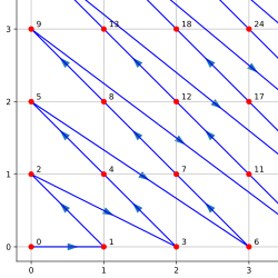
Credit to Wikipedia for the Cantor pairing function image, UCB CS70 for the spiral
Both of these reminded me of how the wallflower fills space in the Cartesian
plane by building outwards from the origin. To use the wallflower’s structure as a pairing
function we would need to find a way to assign an “order” when we place each
square, preferably in a way that complements the recursive nature of its construction.
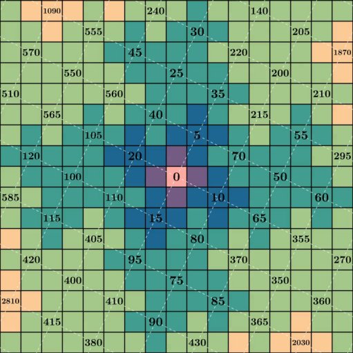
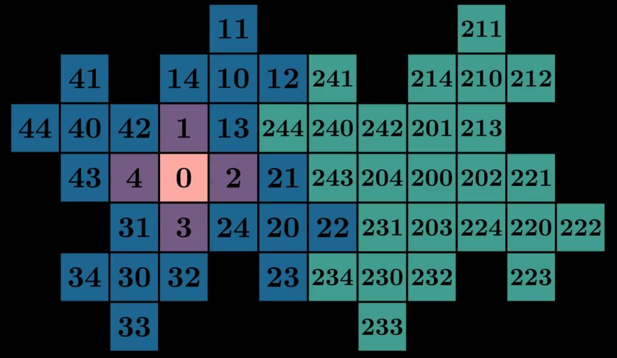
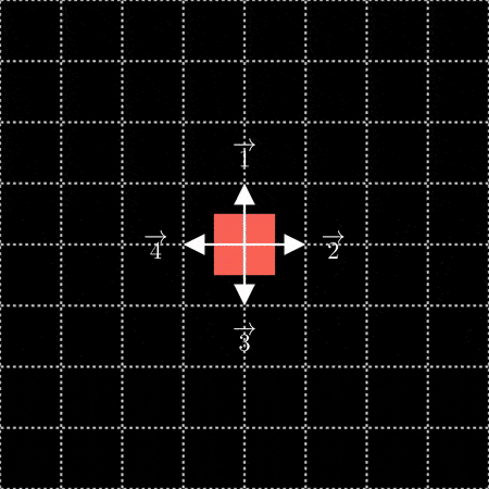
A natural starting point would be to use the center of the fractal as 0. From there we can number
the surrounding four squares added in the first iteration as 1, 2, 3 and 4
in clockwise order:

Now we’re faced with the question of how to label the squares from the next iteration. One
way would be to number them in the order they appear scanning from top down, left to right:
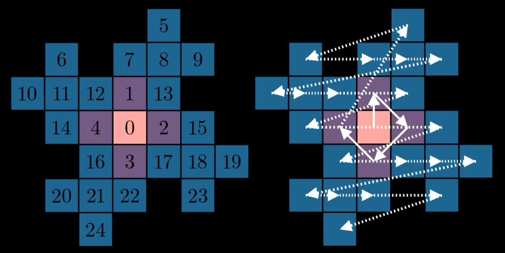
For lack of better words, this doesn’t feel very fractally – the order here seems unrelated to recursive
structure of fractal. What if instead we tried to reuse the “middle out” approach used for
0 to 4? After all, each “petal” is a copy of the first iteration we’ve
already given an ordering to. Reusing the clockwise scheme from 0 to 4 within each blue
petal, and across each blue petal (the dashed lines):
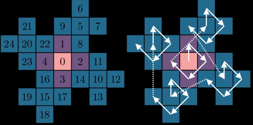
And extending to the next set of petals:
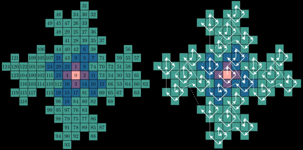
As chaotic as it may look at first glance, a few interesting properties emerge
if we look at the positions of certain numbers. If we isolate our view to just multiples of 5,
a scaled up grid tilted about 27 degrees clockwise is formed:
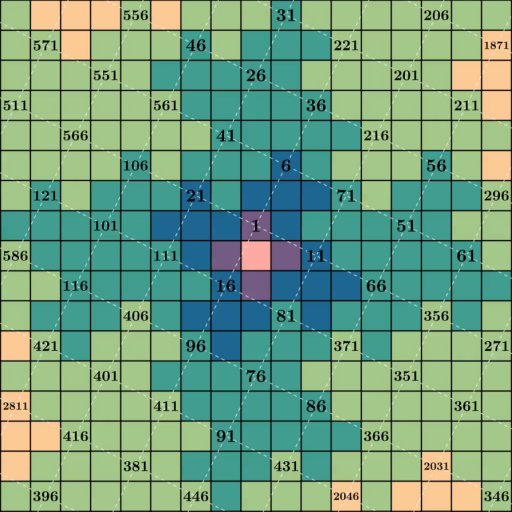
If we only look at the numbers of the form (5n + 1),
we get the previous grid but scooted up by 1 square:
And if we look at just multiples of 25 we get another grid, scaled up even further:
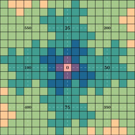
The number 5 appears to have a special relationship with the fractal. The reason becomes
apparent if you look at the number of squares in each iteration. The 0th iteration
is a single square, the first iteration has 5, the second has 25, the third has 125, etc… Since
each iteration is constructed by taking the previous state and adding 4 additional copies,
it scales up by a factor of 5 in each step. Given the special relationship
with multiples of 5 and powers and 5, it’s tempting to redo the labeling while counting
in base 5 instead of base 10. Doing so we get this:
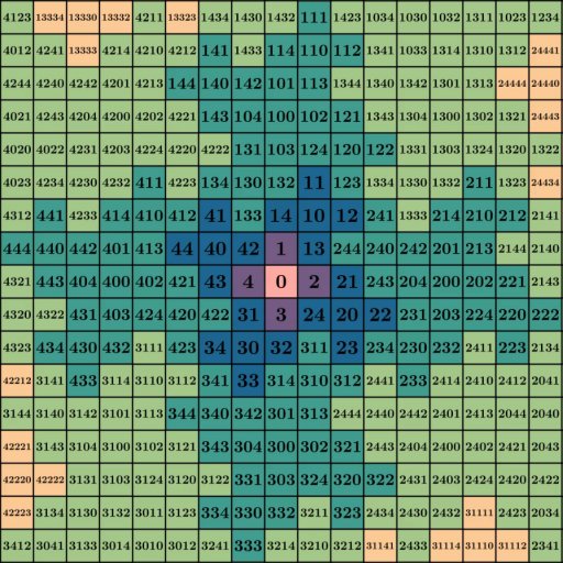
This is a ton of information, but if we focus in on just the iteration 3 pattern and its copy to the right you might
notice something interesting:
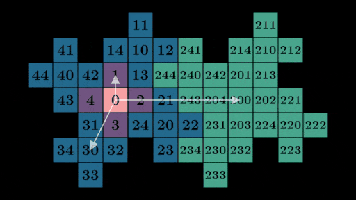
How to add
If you take any number on the left and check 5 spaces to the right, you’ll find
its copy on the teal petal. Comparing the numbers between cells, they always seem to be
the original value plus 200. For example, 5 spaces to the right of
44 you’ll find 244, and 5 spaces to the right of 3 is 203. In some sense, adding 200
seems to encode “shifting” 5 spaces to the right. This “shifting” property isn’t unique to 200
either: consider the positions of 0, 1, 2, 3, and 4 relative to 30, 31, 32, 33, and 34.
If you stare for long enough you might notice by expanding any number, say 231 = 200 + 30 + 1,
we can use each number in the expanded form to find its location on the grid. In this case, we
can find vectors corresponding to 200, 30, and 1 on the grid and add them
together to get the location of 231:
You can test out other numbers using the same strategy of breaking down the number into
its 1s, 10s, 100s, etc… places and adding vectors. Assuming
this works in general, all we need to find the position of any number on the grid is to know the position of each number
in its expanded form, and then add them together. Let’s abuse introduce some notation, defining (vec{n}) as the vector
pointing to where the number (n) sits on the grid. Using our 1 digit values as an example:
(begin{align}
overrightarrow{0} &= begin{bmatrix}
0 \
0 \
end{bmatrix}
end{align},)(begin{align}
overrightarrow{1} &= begin{bmatrix}
1 \
0 \
end{bmatrix}
end{align},)(begin{align}
overrightarrow{2} &= begin{bmatrix}
0 \
1 \
end{bmatrix}
end{align},)(begin{align}
overrightarrow{3} &= begin{bmatrix}
-1 \
0 \
end{bmatrix}
end{align},)(begin{align}
overrightarrow{4} &= begin{bmatrix}
0 \
-1 \
end{bmatrix}
end{align})
With this new notation, we can stare at how “powers of 10” seem to behave:
(begin{align}
overrightarrow{1} &= begin{bmatrix}
0 \
1 \
end{bmatrix}
end{align},)(begin{align}
overrightarrow{10} &= begin{bmatrix}
1 \
2 \
end{bmatrix}
end{align},)(begin{align}
overrightarrow{100} &= begin{bmatrix}
0 \
5 \
end{bmatrix}
end{align},)(begin{align}
overrightarrow{1000} &= begin{bmatrix}
5 \
10 \
end{bmatrix}
end{align},)(begin{align}
overrightarrow{10000} &= begin{bmatrix}
0 \
25 \
end{bmatrix}
end{align},)(begin{align}
overrightarrow{100000} &= begin{bmatrix}
25 \
50 \
end{bmatrix}
end{align})
Looking closely you might pick up on the pattern:
[begin{equation}
overrightarrow{(10^n)} = begin{cases}
5^n begin{bmatrix}
0 \
1 \
end{bmatrix} & text{if } n text{ is even} \
5^{(n-1)} begin{bmatrix}
1 \
2 \
end{bmatrix} & text{if } n text{ is odd}
end{cases}
end{equation}]
This conditional formula was
how I initally wrote the visualization code. However it begged the question:
is there a more elegant way to compute the values without needing a conditional?
Ideally we want a transformation we could repeatedly apply to scale and rotate a vector
based on the value of (n), i.e. a matrix raised to the power of (n). With some fiddling around, we can find the matrix (M) and its powers:
(M = begin{bmatrix}
-2 & 1 \
1 & 2\
end{bmatrix},)(M^2 = begin{bmatrix}
5 & 0 \
0 & 5\
end{bmatrix},)(M^3 = begin{bmatrix}
-10 & 5 \
5 & 10\
end{bmatrix},)(M^4 = begin{bmatrix}
25 & 0 \
0 & 25\
end{bmatrix}, text{etc…})
Which conveniently matches the values we’re expecting without needing a conditional in the equation:
[overrightarrow{(10^n)} = M^noverrightarrow{1} = begin{bmatrix}
-2 & 1 \
1 & 2\
end{bmatrix}^nbegin{bmatrix}
0 \
1 \
end{bmatrix}]
Similarly we can set up equations for the other possible digits:
[begin{align}
overrightarrow{(2 cdot 10^n)} &= M^noverrightarrow{2} = begin{bmatrix}
-2 & 1 \
1 & 2\
end{bmatrix}^nbegin{bmatrix}
1 \
0 \
end{bmatrix}
newline
overrightarrow{(3 cdot 10^n)} &= M^noverrightarrow{3} = begin{bmatrix}
-2 & 1 \
1 & 2\
end{bmatrix}^nbegin{bmatrix}
0 \
-1 \
end{bmatrix}
newline
overrightarrow{(4 cdot 10^n)} &= M^noverrightarrow{4} = begin{bmatrix}
-2 & 1 \
1 & 2\
end{bmatrix}^nbegin{bmatrix}
-1 \
0 \
end{bmatrix}
end{align}]
If you blur your eyes with the tears shed over the cursed notation, you might
make out a connection to number systems such as base 5 or base 10.
Similar to how in base 10 the number 1234 would expand to:
[begin{aligned}
1234 &= 10^3 cdot 1 + 10^2 cdot 2 + 10^1 cdot 3 + 10^0 cdot 4
newline
1234 &= 1000 + 200 + 30 + 4
end{aligned}]
And in base 5:
[begin{aligned}
1234_5 &= 5^3 cdot 1 + 5^2 cdot 2 + 5^1 cdot 3 + 5^0 cdot 4
newline
1234_5 &= 1000_5 + 200_5 + 30_5 + 4_5
end{aligned}]
We can use the matrix (M) as our base, and vectors as our digits to encode positions
in the fractal:
[begin{aligned}
overrightarrow{1234} &= M^3overrightarrow{1} + M^2overrightarrow{2} + M^1overrightarrow{3} + M^0overrightarrow{4}
newline
overrightarrow{1234} &= overrightarrow{1000} + overrightarrow{200} + overrightarrow{30} + overrightarrow{4}
end{aligned}]
We’ve stumbled upon a number system with a matrix base and vector digits, rather than scalars!
Counting up from 0 we can get a feel for the how the number system connects to the structure
of the fractal:
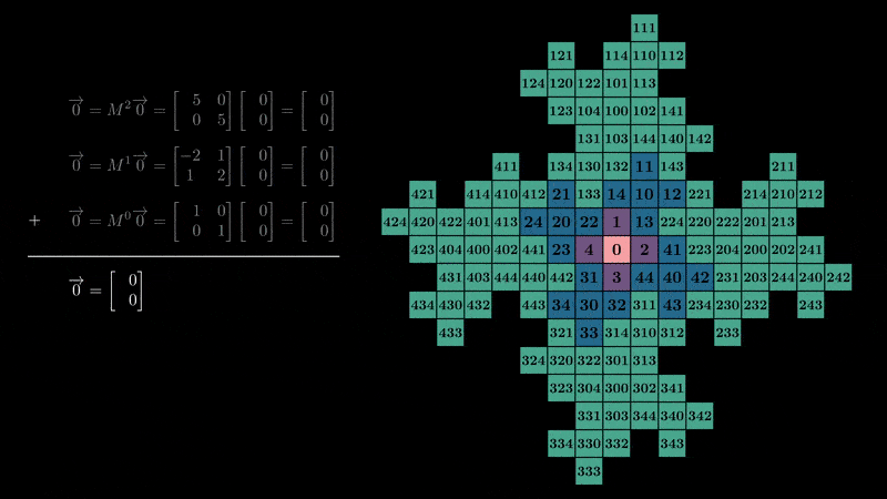
Determinants
You may have noticed (20) and (40)
have switched positions compared to our original numbering. This is because our choice
of (M) has a negative determinant (det(M) = -5), which means it has the side effect of “flipping” the
orientation of space each iteration. Now that we know our fractal is linked to linear algebra,
we can visualize the connection by overlaying scaled grids representing how powers of (M) act on our “digit vectors”
(vec{1}), (vec{2}), (vec{3}) and (vec{4}) a la 3Blue1Brown.
To avoid the flipping behavior we would need to pick a matrix with a positive determinant,
for example:
[M^prime = begin{bmatrix}
2 & 1 \
-1 & 2\
end{bmatrix}]
[det(M^prime) = 5]
Visualizing this new choice of matrix:
Instead of “flipping” and realigning with the axes every other iteration, this choice of
base continually rotates our “digit vectors” clockwise.
Wait, didn’t we see a version of the fractal like this way back at the start with the L-System?
Sure enough, using (M^prime) as our base reproduces the L-System version.

Mystery solved! The two fractals are almost the same, but the one on my wall is generated using
(M) where (det(M) = -5), while the more common one is generated from (M^prime)
where (det(M^prime) = 5). The choice of matrix also sheds some light on where the seemingly
arbitrary “about 27 degrees” comes from. You may have noticed the absolute value of both
determinants is (5), which conveniently matches the way the fractal increases in size by a factor
of 5 each iteration. If we picked a matrix with a larger determinant, our “digit vectors” would
grow too quickly and leave behind “empty space” each iteration. For example adjusting (M) to give
it a determinant of (-6) results in:

Meanwhile if we pick a matrix with a smaller determinant, our “digit vectors” would grow too
slowly and iterations would overlap. Adjusting (M) to give it a determinant of (-4):
So ostensibly we want a matrix base with determinant (pm 5). Additionally, we want our
matrix to have integer entries to ensure it always maps our digit vectors onto
whole number coordinates. It just so happens the vector (leftlangle 1, 2 rightrangle)
has integer entries and magnitude (sqrt{5}), meaning we can use it and one of
its 90 degree rotations as the columns of our matrix to satisfy the determinant
and whole number constraint. Computing the angle of this vector we get (arctan{frac{2}{1}} approx 63.43^circ),
i.e. “about 27 degrees” away from the y-axis.
How to add part 2
You may have noticed vector addition fails horribly in most cases other than
the expanded form ones, e.g. (vec{2} + vec{2} neq vec{4}). This is expected, since the choice of (2) and (4)
were to help make the connection to base 5 number systems but unrelated to the
actual direction the vectors point. It might be more appropriate to refer to 1 through 4
as up ((vec{1})), right ((vec{2})), down ((vec{3})), and left ((vec{4})). As you
might expect, opposite directions cancel eachother out, i.e. (vec{1} + vec{3} = vec{2} + vec{4} = vec{0}).
But what about other combinations of additions? By looking closely at the base 5 numbering and following where
combinations of unit vectors point:

We can build up a table based on where it appears the sum of unit vectors would fall:
| (+) | (overrightarrow{0}hspace{5pt}) | (overrightarrow{1}hspace{5pt}) | (overrightarrow{2}hspace{5pt}) | (overrightarrow{3}hspace{5pt}) | (overrightarrow{4}hspace{5pt}) |
|---|---|---|---|---|---|
| (overrightarrow{0}hspace{5pt}) | (overrightarrow{0}) | (overrightarrow{1}) | (overrightarrow{2}) | (overrightarrow{3}) | (overrightarrow{4}) |
| (overrightarrow{1}hspace{5pt}) | (overrightarrow{1}) | (overrightarrow{14}) | (overrightarrow{13}) | (overrightarrow{0}) | (overrightarrow{22}) |
| (overrightarrow{2}hspace{5pt}) | (overrightarrow{2}) | (overrightarrow{13}) | (overrightarrow{41}) | (overrightarrow{44}) | (overrightarrow{0}) |
| (overrightarrow{3}hspace{5pt}) | (overrightarrow{3}) | (overrightarrow{0}) | (overrightarrow{44}) | (overrightarrow{32}) | (overrightarrow{31}) |
| (overrightarrow{4}hspace{5pt}) | (overrightarrow{4}) | (overrightarrow{22}) | (overrightarrow{0}) | (overrightarrow{31}) | (overrightarrow{23}) |
The table is symmetric across the diagonal meaning addition is commutative, as expected
for vector addition. More importantly, several additions result in 2 digit values. While it might
not seem like a big deal, it means when doing larger additions we have to worry about
carrying over values to the next digit. For example, if we want to find the number directly
above 22, we can compute (overrightarrow{22} + overrightarrow{1}). Using
traditional long addition and carrying notation:
[begin{array}{cccc}
& overset{1}{vphantom{0}} & overset{1}{2} & 2 \
+ & & & 1 \
hline
& 1 & 3 & 3 \
end{array}]
If you’re a bit confused, remember (overrightarrow{2} + overrightarrow{1} = overrightarrow{13}).
And if you’re suprised this works at all, join the club! Since this is a blog post and not a proof,
I leave sanity checking this addition scheme works in general to the reader.
The concept of using things outside of (mathbb{N}) in a number system wasn’t totally unfamiliar thanks to Balanced Ternary
which uses (-1), (0), and (1) as digits, and a base of (3). If you imagine balanced
ternary as being 1 dimensional along the x-axis, the wallflower can be seen as its 2D analog
by adding two new digits to account for the positive and negative directions of the y-axis.
An alternative scheme for generalized balanced ternary
already exists, and generalizes to any number of dimensions using lattices of permutahedrons
(at least from what I’ve been able to dig up). In 2 dimensions, this ends up being the hexagonal lattice:
Visualization of generalized balanced ternary in 2D using hexagons from Wikipedia. See also Gosper Curve,
which is like a hexagonal wallflower.
Another exotic number system is Quater-imaginary Base,
which uses the imaginary value (2i) as its base, and (0), (1), (2) and (3) as digits.
If you imagine complex numbers as vectors, and imagine (2i) as a matrix that performs a scale and rotation,
we can convert this number system into our cursed notation:
(M_{2i} = begin{bmatrix}
0 & -2 \
2 & 0\
end{bmatrix},)(overrightarrow{0} = begin{bmatrix}
0 \
0 \
end{bmatrix},)(overrightarrow{1} = begin{bmatrix}
1 \
0 \
end{bmatrix},)(overrightarrow{2} = begin{bmatrix}
2 \
0 \
end{bmatrix},)(overrightarrow{3} = begin{bmatrix}
3 \
0 \
end{bmatrix})
Alternatively, we can convert the positive determinant matrix (M^prime) from earlier into its
complex number equivalent to get a base (2+i) number system. Balanced base 2+i (and some gratuitous fractals)
by Timothy James McKenzie Makarios explores this concept. I ran into this while looking for visualizations of
quater-imaginary base on Google images for this section, only to realize this connection had been
made back in 2016. Somewhat embarassingly I found this after I made the animation at the
start, only to find the author had already beaten me to that as well, although
using the (M^prime) version of the fractal instead of (M) (as far as I know (M)
cannot be encoded as a complex number).
When I realized the matrix base number system worked at all I started
searching around to see if anyone else had made the connection between fractals, tesselations, linear algebra
and number systems. Digging around:
- Project BinSys led by Attila Kovács
is focused on finding matrix bases specifically where the determinant is 2, for a generalized form of binary. - Replicating Tesselations
by Andrew Vince does all the rigorous math stuff to formalize what I’ve been trying to
describe through vigorous handwaving, and generalizes to any lattice rather than just (mathbb{Z}^2).- Here you can also find proofs for the alternative way to generalize balanced ternary
into higher dimensions.
- Here you can also find proofs for the alternative way to generalize balanced ternary
Speaking of handwaving: the next section is now fully in the territory of “things I
started to think about a week ago when I started writing this,” so any semblance of rigor
that came from having many years to think about the problem is out the window. Instead
I’ll be relying on my mental model of linear algebra, which is “if it sounds like it’s true
and looks like it’s true, it’s probably true.”
To go even further beyond
Middle school me was really into Minecraft, so naturally I always wondered: would the fractal work with
cubes? Specifically, is there a way to create a 3D version of the fractal by
starting with cube and copying outwards in groups of six to form a “3D plus”? This mostly
comes down to what properties we want to include when we generalize to a 3×3 matrix. The
ones that beckoned to me from the ether are:
- All of the entries in the matrix must be integers. This is needed so when we apply
the matrix base to our vector digits (6 unit vectors sitting on the axes) they still
have integer values for each component. In the Vince paper this is formalized as “endomorphism of (Lambda)”,
i.e. a mapping from the lattice (Lambda = mathbb{Z}^3) back onto itself. - Each column vector in the matrix should have a Hamming distance of 3 from the origin.
This constraint ensures the 6 copies of the “3D plus” we create on the second
iteration don’t overlap with the original centered on the origin, but are near enough to still
be adjacent to it. - We want a matrix with determinant (pm)7. Since each iteration of the fractal adds 6 new copies,
we increase the size of the fractal by 7 times each step. If we want to “pack” together these
copies efficiently we need to make sure the matrix we apply scales up
inputs by a factor of 7 as well.
Brute force searching through triplets of vectors with Hamming distance of 3, we get this nifty 3×3
matrix that checks all of the boxes:
[begin{bmatrix}
2 & -1 & 0 \
-1 & 0 & 2 \
0 & -2 & 1 \
end{bmatrix}]
Visualizing gives us:
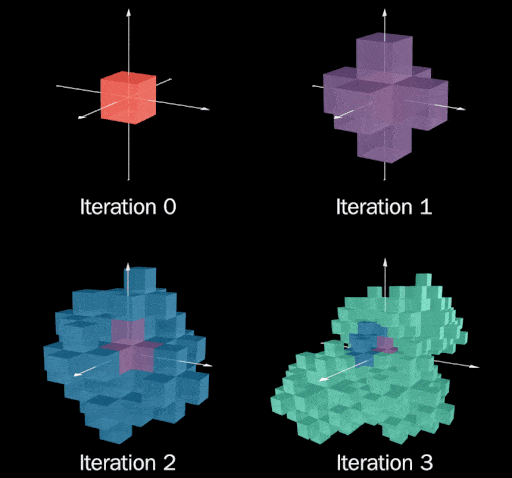
Wow, it looks terrible! One problem that stands out immediately is later iterations seem to be “smooshed”
resulting in spots where previous iterations are exposed.
Looking closely at iteration 2, you might notice we can comb over the bald spots
by adding two more “3D pluses” centered on (leftlangle 1, 1, 1rightrangle) and (leftlangle-1, -1, -1rightrangle).
Here we added two new pluses marked in yellow, and visualize the location of the centers
of all 8 pluses. For a bandaid fix it feels like it works a little too well. Looking at just
the center points of our 8 new pluses they are arranged like the vertices of a warped cube.
I’m still not entirely sure what to make of this, although it feels like it’s related to
the fact that cubes (8 vertices, 6 faces) are the dual solid to octahedrons (6 vertices, 8 faces).
It’s obviously tempting to try to take this new cube and make 6 copies of it, but to avoid
derailing this post too much let’s save that for another day.
Visually, the problem with iteration 2 seems to be that the 3D pluses aren’t placed symmetrically
around the center, causing the fractal to expand in a non-uniform way. Manually trying to find a more symmetrical
arrangement of 6 pluses is tricky, feeling a bit like trying to comb a hairy ball.
A sufficient (and possibly necessary) condition to prevent the smooshing behavior is
to pick a matrix where each column is mutually orthogonal and has the same magnitude. I suspect if
we include this with the prior constaints it’s impossible to satisfy in 3D. Each integer valued
column vector would need a magnitude of (sqrt[3]{7}), so given that (x, y) and (z) are integers,
we must solve:
[sqrt{x^2+y^2+z^2} = sqrt[3]{7}]
[x^2 + y^2 + z^2 = 7^{2/3}]
This can never be true since the left hand side is always an integer, while the right hand
side is irrational. Luckily, if we go up to four dimensions the math works out in our favor. In 4 dimensions
the components of each vector must satisfy:
[sqrt{x^2 + y^2 + z^2 + w^2} = sqrt[4]{9}]
[x^2 + y^2 + z^2 + w^2 = 3]
Which works if we let 3 out of 4 of the entries to be (pm 1),
and set the last to (0). It turns out there’s a plenty of space in hyperspace, giving us many
possible matrices with columns of this form that satisfy all previous conditions. The
following matrix has one extra property that we’ll cover briefly near the end:
[begin{bmatrix}
0 & -1 & -1 & -1 \
1 & 0 & -1 & 1 \
1 & 1 & 0 & -1 \
1 & -1 & 1 & 0 \
end{bmatrix}]
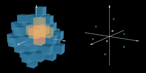
Now that we have a suitable matrix, we can attempt to visualize our 4D fractal.
One way to do this is to take 3D “slices” of 4D space by fixing the
value of (w):
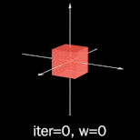
It turns out the base case is boring regardless of how many dimensions we give it. Moving
on to iteration 1:
From here you can get a better feel for how the visualization works. The purple cubes on the
left and right that appear to be sitting at the origin are really at the ((x,y,z,w))
coordinates of ((0,0,0,-1)) and ((0,0,0,1)) respectively.

We can see parts of iteration 1 still poking through in iteration 2, which is concerning given this
was a symptom of the squishing behavior we saw in 3D. However looking closely, the squishing
behavior doesn’t seem as bad yet. If you really twist your mind around the concept of 4
dimensions, you might be able to see that while the two pluses in (w=0) don’t
seem to be balanced, there are 3 pluses sitting to the left ((w=-1)) and 3 more to the
right ((w=1)) that you could imagine as being orthogonal to the (w=0) ones. The trios
of cubes sitting at each side ((w=pm 2)) are part of the 4D pluses that poke through
the 4th dimension into the slices on the ends.

My main takeaway from this is that while iteration 2
can still be seen, iteration 1 has now been completely covered.
Technically iteration 3 extends farther out in the (w) dimension, but at this point it’s
difficult to comprehend the fractal anyway. I imagine this is the sort of thing my higher dimensional analog would
put up on the 4D hypersurface of their room’s 5D walls to admire in its full glory, so I’m dubbing it “the orthotopeflower.”
Unfortunately my apartment is measured in square feet and not hypercubic feet, so
it’s difficult for me to fully appreciate it. There are a couple of issues with the “3D slices”
approach of visualizing in 4D:
- It extends way too quickly in the horizontal direction, wasting precious screen
(or wall) real estate. Notably in iteration 3 we
need to add 2 more slices to each side to visualize the whole thing. - My inferior 3 dimensional eyes can’t see the interior of 3D objects (unlike how I’m
able to see the interior of colored in 2D squares on a piece of paper), making it
hard to fully appreciate the structure.
To get around both of these limitations we can use the following 7×7 grid of 7×7 grids to visualize it
a la the very first animation of this post:

Here’s a static image of the last iteration if you want to admire it. If this isn’t nice, what is?
Each smaller grid shows a slice of -3 to 3 on the x and y axes. The “grid of grids” represent
-3 to 3 along the z and w axes. Whenever a square crosses from one small grid
to another it’s really being translated through the z or w axis. Squares that appear to
fade in or fade out are moving in or out of the 7x7x7x7 “viewing window” in 4 dimensions.
Compared to the line of 3D slices, this approach uses screen real estate a bit better
(growing as a square instead of in a line), and lets you see the interior of the entire
fractal without obscuring previous iterations. Plus this design would go nicely with
the existing fractal on my wall.
If we’re willing to discard all of the flourishes from the animation and assign 1 pixel
per tile in the fractal we can increase our viewing window up to 31x31x31x31:
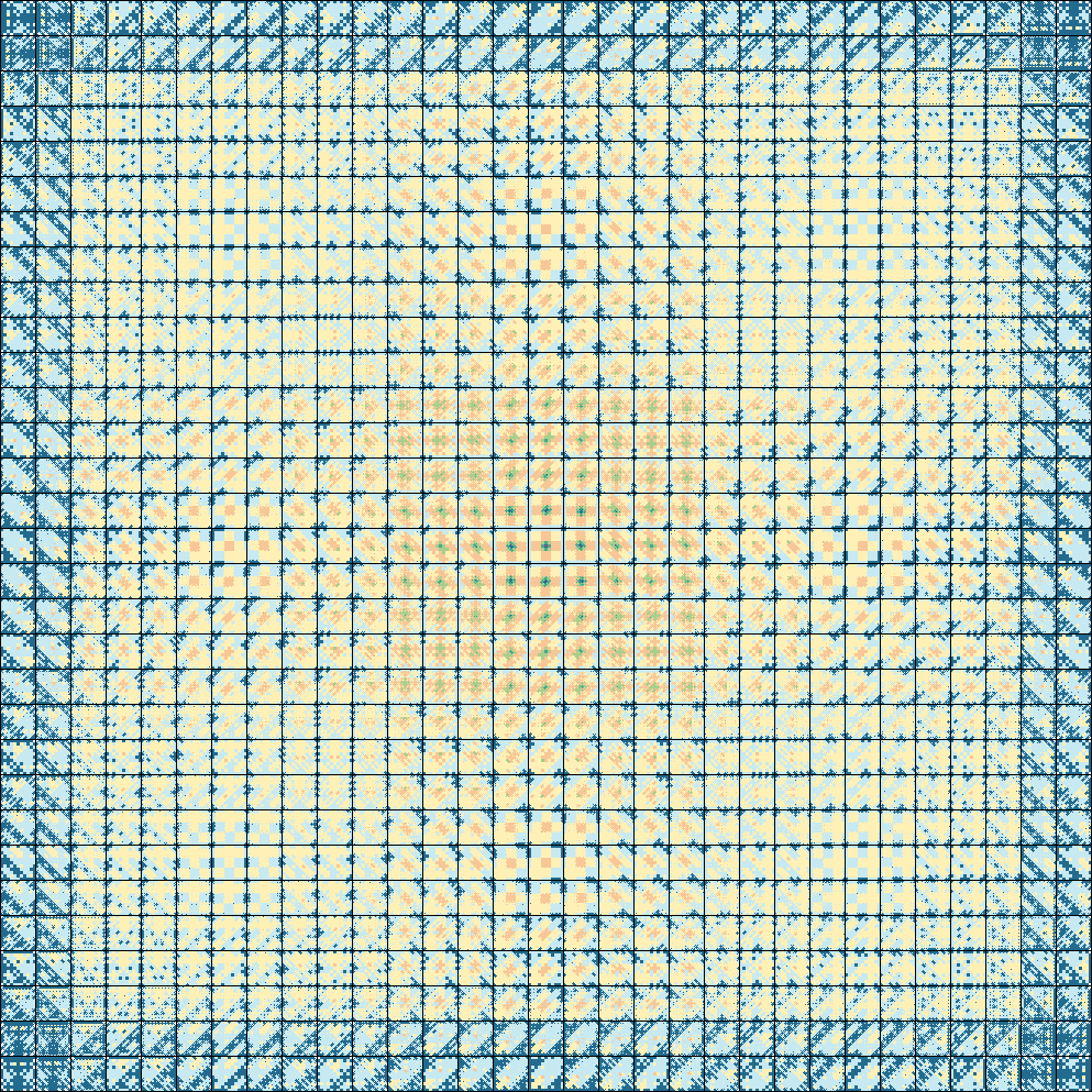
It’s a lot to take in, but at the very least seems to confirm that the fractal consistently
expands outwards without excessive smooshing like we saw in 3D. And personally, I think
it would make a lovely quilt or picnic blanket. In particular these slices near the very
center are remarkably pleasant:

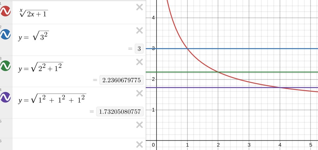
A natural question is if we can continue into higher dimensions. Sadly I suspect the
answer is no. Applying all our constraints from earlier we need a dimension (d) such that:
(sqrt[d]{2d+1} in)({sqrt{3^2}, sqrt{1^2 + 2^2}, sqrt{1^2+1^2+1^2}})
The left hand side is the magnitude each column vector needs to be for a matrix with (d) mutually
orthogonal columns to have determinant (2d+1) so that it scales inputs enough to fit the (2d) copies added each iteration.
The right hand side is the set of possible magnitudes of integer valued vectors that have a Hamming distance of 3 away from the origin, so
the copies created in the second iteration touch but don’t intersect with the first iteration.
Graphing this, it looks like the only dimensions where these can be satisifed are 1 (balanced
ternary), 2 (the wallflower/quadratic flake), and 4 (the orthotopeflower).
Finally, as mentioned earlier, the choice of matrix to use as the base of our 4D number system was special. In particular
it encodes the quaternion (i+j+k), meaning similar to quater imaginary base we now
have a way to encode quaternions in “balanced nonary quaternion base”. In this scheme
the 9 possible digits are (0), (pm1), (pm i), (pm j) and (pm k), with base (i+j+k). Since I’m not too familiar
with quaternions and still not entirely sure if this actually works, I’ll be delegating
this problem to a future version of me who knows more math. This strategy seemed to work
pretty well last time.
Closing thoughts
I once had a dream about a post-scarcity society that had to work around the problem of
people not having any motivation to do anything, since all their basic needs were met.
To give people something to do, every few years everyone over a certain age was expected
to report on something beautiful they learned or discovered about the world, otherwise
they’d be turned into soylent or something (Note: post-scarcity (neq) utopia). Anyway, I’d like to
imagine the discovery of a strange flower with jigsaw-like petals blooming endlessly across 4
dimensional space would be enough to keep me off the chopping block for awhile.
I finally got around to this in an attempt attempt to reignite some passion for math and programming
after a period of burnout. It turns out my younger
self left behind the perfect gift in the form of a scavenger hunt across the domains of fractals, number systems,
linear algebra and higher dimensions. It makes me curious about how many other interesting
ideas other people have lying around in plain sight as sketches or To Do’s.
If this post comes off as a bit rambly from the many twists and turns between domains it’s
because I tried to follow the path I took while haphazardly picking up and forgetting
about the problem over the years. There are a handful of spots where you might ask “how did you know
doing this specific thing would lead to that?” The simple answer is I had no clue if any of this
would lead anywhere, I just tried different things on a whim and this post outlines the parts that stuck.
Hopefully by writing and visualizing my lines of reasoning I’m able to make the connections a bit more accessible
for future fractal fiddlers finding themselves falling face first down the same rabbit hole.
As a final twist, an astute reader may have
noticed none of the visualizations made for this post
matched the fractal on my wall in the post’s thumbnail. The 4th iteration (green) is copied about 27
degrees in the wrong direction:

In a fun case of “why do I remember this, but not what I ate for dinner 2 days ago,” I
remember my exact reasoning for doing this over a decade ago: I thought the fractal
would unalign itself from the cardinal directions if I always tilted it off the axes in the
same direction. As we saw earlier with (M) vs (M^prime) my intuition to compensate for tilt almost made sense, other
than the fact it already corrects itself in alternating steps. I was a bit
embarassed about this until I remembered even Donald Knuth
made a wrong turn when putting up a fractal on his wall.
Fools rarely differ!

