


Tony??Phillips is an experienced Microsoft Office user with a dual-honors degree in Linguistics and Hispanic Studies. Prior to starting with How-to Geek in January 2024, he worked as a document producer, data manager, and content creator for over ten years, and loves making spreadsheets and documents in his spare time.
Tony is also an academic proofreader, experienced in reading, editing, and formatting over 2.8 million words of personal statements, resumes, reference letters, research proposals, and dissertations. Before joining??How-To Geek, Tony formatted and wrote documents for legal firms, including contracts, Wills, and Powers of Attorney.
Tony is obsessed with Microsoft Office! He will find any reason to create a spreadsheet, exploring ways to add complex formulas and discover new ways to make data tick. He also takes pride in producing Word documents that look the part. He has worked as a data manager in a secondary school in the UK and has years of experience in the classroom with Microsoft PowerPoint. He loves to encounter problems in Microsoft Office and use his expertise and legal-level training to find solutions.
Outside of the Microsoft world, Tony is a keen dog owner and lover, football fan, astrophotographer, gardener, and golfer.
When you apply Microsoft Excel’s percentage number format to a cell already containing a number, it multiplies the value by 100. This can be frustrating, as there’s apparently no easy way to stop this from happening. Until now!
Imagine you want to turn all the gradient values in column B in the table below into percentages.

However, if you select all the cells containing these values and click the “%” icon in the Number group of the Home tab on the ribbon, all the numbers are multiplied by 100, resulting in larger percentage values than you intended. This is because Excel assumes your percentages are expressed as a fraction of 100, with 1 equating to 100%, 0.5 equating to 50%, and so on.

There are various ways to rectify this, but they usually require you to insert a helper column or type a formula. However, there’s an easier and quicker fix.
With the numbers in column B in their original format, type 1% into a blank, unformatted cell, and press Enter. Then, go back to that cell, and press Ctrl+C to copy it. The aim is to multiply all the numbers you want to convert by 1% (or 0.01) to revert them to their previous values, while also adding the percentage symbol to each.

To do this, with the 1% cell still copied, select the cells containing the values you want to convert from whole numbers into percentages. If your data is formatted as an Excel table, hover over the column header until you see a small, black down arrow, and click to select the whole column.
On the other hand, if your data is in regular cells, navigate to the highest data cell in the column, and press Ctrl+Shift+Down.

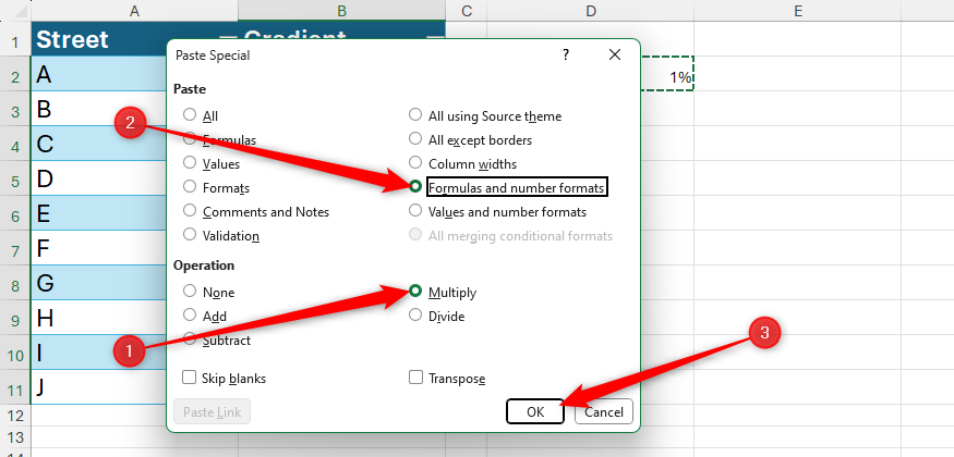
Now, press Ctrl+Alt+V to launch the Paste Special dialog box. Alternatively, click the “Paste” down arrow in the Home tab on the ribbon, and select “Paste Special.”

In this case, you want to perform the multiplication operation, so check the “Multiply” radio box or press M. Also, you want to preserve the direct formatting of the cells in column B while adopting the percentage formatting from the cell you’ve copied, so check “Formulas And Number Formats” in the Paste section, or press R. Then, click “OK” or press Enter.
Now, all the values are converted to percentages, and their original formatting has been retained.

By default, Excel expresses percentages with no decimal places. So, with the newly converted percentages still selected, click the “Increase Decimal” icon (a series of zeros with a blue left arrow) in the Number group of the Home tab on the ribbon to add decimal places. On the other hand, click “Decrease Decimal” to reduce the number of decimal places.
Since the influencer cell containing 1% is not linked in any way to the values you just converted, you can clear its contents and percentage formatting. To do this, select the cell, click the “Clear” icon in the Editing group of the Home tab on the ribbon, and click “Clear All” from the drop-down menu.

If you’re working in an Excel table, when you add data to the next blank row at the bottom or rows inserted in the center, the new cells in column B automatically adopt the percentage number format and decimalization you applied to the other cells in the same column, so you can type a whole number safe in the knowledge that it will be presented correctly and consistently.

This is also the case for data in regular ranges, provided “Extend Data Range Formats And Formulas” is checked in the Advanced section of the Excel Options dialog box. You can launch this dialog box by clicking Home > Options or pressing Alt > F > T.

Alongside the standard number format options in Microsoft Excel, such as the percentage, text, and general number formats, you can apply a custom number format to hide cell values, replace zeros with a dash, turn certain values to text, color numbers based on their values, and much more.
Microsoft 365 Personal
- OS
-
Windows, MacOS, iPhone, iPad, Android
- Free trial
-
1 month
Microsoft 365 includes access to Office apps like Word, Excel, and PowerPoint on up to five devices, 1 TB of OneDrive storage, and more.

